CMCC SPS3.5 Operational Seasonal Prediction System - Synthetic System Description

Table of Contents
Introduction
The CMCC SPS3.5 Operational Seasonal Prediction System
Dissemination
CMCC-SPS3.5 participation in Multi-Model Ensembles
Where to find additional information
References

Introduction

The purpose of this document is to provide a description of the new version of the operational CMCC (Euro-Mediterranean Center on Climate Change) SPS3.5 Seasonal Prediction System/Model(s), version which has replaced in operations the former version SPS3, starting from the operational forecast of October 1st, 2020. The new version differs from the previous one essentially only for the horizontal resolution of the atmospheric model component (CAM 5.3), plus a number of somewhat minor details which will be described below. All hindcasts previously available (1993-2016) have also been rerun, for the same dates, at the new, higher, atmospheric model resolution, all other system characteristics having remained essentially the same. The CMCC Seasonal Prediction System has been developed at CMCC on the basis of the models described below and routinely performs forecasts at the seasonal time scale which are provided, among others, to Copernicus-C3S and will be soon provided to WMO LC-LRFMME (WMO Lead Centre for Long-Range Forecast Multi-Model Ensemble). A selection of products and verifications are also available via this dedicated CMCC public website https://sps.cmcc.it/.

The CMCC SPS3.5 Operational Seasonal Prediction System

The acronym and full name of the System is CMCC-SPS3.5, i.e. Euro-Mediterranean Center for Climate Change - Seasonal Prediction System, Version 3.5. The System is based on a comprehensive coupled Ocean-Atmosphere Global Climate Model, complemented by a number of additional modules.

Description of the Operational Prediction System

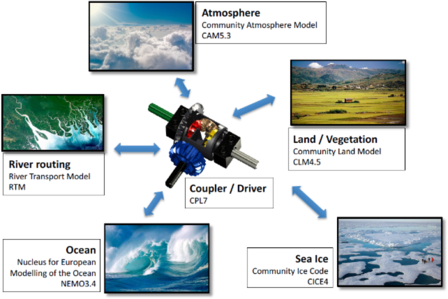
The current version of the CMCC-SPS3.5 System consists of several independent but fully coupled model components simultaneously simulating the Earth’s atmosphere, ocean, land, sea ice and river routing, together with a central coupler/driver component that controls data synchronization and exchange (see the sketch of Figure 1).

The CMCC-SPS3.5 atmospheric, land surface, sea ice and river routing model components are based on CESM, the NCAR Community Earth System Model version 1.2.2 (in their CAM5.3, CLM4.5, CICE4 and RTM versions, respectively). A detailed description of such models is given in Hurrell et al. (2013) and references therein. The ocean component is based on NEMO, the European Nucleus for European Modelling of the Ocean model, in its 3.4 version; for a detailed description, see Madec et al. (2008). For a first evaluation of the former system CMCC-SPS3 performance (bias and skill), see Sanna et al. (2018) and for some further technical information on SPS3.5, see Gualdi et al. (2020).

The System is operated monthly in Ensemble seasonal mode (6-month predictions) and is completed by a database of monthly ensemble hindcasts covering the period 1993-2016 which can be used to evaluate the performance of the System and to apply bias removal techniques from operational forecasts. The first operational seasonal forecast run produced for Copernicus C3S with the previous System Version, CMCC-SPS3, and contained in the CDS, was initiated from April 1st, 2018, 00:00 UTC and continued monthly hereafter, from the first day of every month, up to September 1st, 2020. All further monthly seasonal forecasts (all with a forecast horizon of six months) from January 1st, 2017 until March 1st, 2018 have also been produced and are also available from CMCC as POPs, Pre-Operational Predictions. From October 1st, 2020, CMCC-SPS3 has been replaced in operations by CMCC-SPS3.5. All these forecasts and hindcasts constitute, together, a continuous database of monthly ensemble seasonal (6-month) forecasts from January 1st, 1993 up to the present date.

Figure 1 – General scheme of the CMCC-SPS3.5 fully coupled Seasonal Prediction System

Atmosphere

The atmospheric component of CMCC-SPS3.5 is the Community Atmosphere Model version 5 (CAM5.3, see Neale et al., 2010 for a description of the model macrophysics) which can be configured to use a spectral element, a finite volume, a spectral Eulerian or a spectral Semi-Lagrangian dynamical core, see Dennis et al. (2012) and Neale et al. (2010). The atmosphere implemented in CMCC-SPS3.5 is hydrostatic and uses the Spectral Element dynamical core (a formulation of the spectral element method using high-degree hybrid polynomials as base functions can be found in Patera, 1984), with a horizontal resolution of ½° (about 55 km), 46 vertical levels up to about 0.3 hPa. A Hyperviscosity term is included in order to damp the propagation of spurious grid-scale modes (Ainsworth & Wajid, 2009).

The integration time-step of the full physics is 30 minutes while, as far as the dynamical core is concerned, the time-step of the “tracer” advection is 225 seconds (1/8 of the physics time-step) and the time-step of the fluid-dynamics is 56.25 seconds (1/32 of the physics time-step).

A description of the treatment for stratiform cloud formation, condensation, and evaporation macrophysics is given in Neale et al. (2010). A two-moment microphysical parameterization (Morrison and Gettelman, 2008; Gettelman et al. 2008) is used to predict the mass and number of smaller cloud particles (liquid and ice), while the mass and number of larger-precipitating particles (rain and snow) are diagnosed. Cloud microphysics interacts with the model’s greenhouse gas concentration, where observed yearly values are specified before 2005 and CMIP5 protocol concentrations (scenario RCP8.5) are used after 2005, see IPCC (2013). Differently from the standard version of CAM5.3, in CMCC-SPS3.5 (as it was also in CMCC-SPS3) the aerosol distribution does not evolve in time through the CAM modal aerosol model (MAM) but is taken from a fixed climatology (referring to year 2000). A Rapid Radiative Transfer Model for GCMs (RRTMG; Iacono et al., 2008, Bretherton et al., 2012, Liu et al., 2012) is used to calculate the radiative fluxes and heating rates for gaseous and condensed atmospheric species. A statistical technique is used to represent sub-grid-scale cloud overlap (Pincus et al., 2003). Moist turbulence (Bretherton and Park, 2009) and shallow convection parameterization schemes (Park and Bretherton, 2009) are used to simulate shallow clouds in the planetary boundary layer.

The process of deep convection is treated with a parameterization scheme developed by Zhang and McFarlane (1995) and modified with the addition of convective momentum transports by Richter and Rasch (2008) and a modified dilute plume calculation following Raymond and Blyth (1986, 1992). Moist convection occurs only when there is convective available potential energy (CAPE) for which parcel ascent from the sub-cloud layer acts to destroy the CAPE at an exponential rate using a specified adjustment time scale.

The physics package includes a parameterization of convective, frontal and orographic gravity wave drag (GWD) following McFarlane (1987), Richter et al (2010) and Richter et al. (2014). The convective GWD efficiency is adjusted to produce a QBO period in the lower stratosphere closer to observations.

The turbulent surface drag due to unresolved orography is taken into account by the Turbulent Mountain Stress (TMS) scheme. Details on this parameterization can be found in Neale et al. (2012), Richter et al. (2010) and Lindvall et al. (2016). Vertical diffusion of heat and momentum is parameterized following Bretherton and Park (2008), with the so-called “University of Washington Moist Turbulence scheme” (UWMT). Inside UWMT the effect of turbulence is represented by a down-gradient diffusion term.

This version of CAM5 uses a modified vertical grid that with 46 vertical levels and a model top at 0.3 hPa.

The increase of atmospheric model resolution from 1° (SPS3) to ½° (SPS3.5) required not only a change of the dynamical core time-step, but also a readjustment (retuning) of surface friction, vertical diffusion and GWD control parameters as outlined below in Sect. 2.5.2.

Atmospheric model	CAM5.3
Dynamics	Hydrostatic, based on a continuous Galerkin spectral finite-element method (basis functions: high degree hybrid polynomials).
Physics	Deep moist convection, stratiform clouds, condensation and evaporation macrophysics, two-moment microphysical parameterization (liquid and ice), orographic, frontal and convective GWD, surface friction and free-atmosphere vertical diffusion. Rain and snow diagnosed, cloud microphysics-GH gases interaction (GH gases concentration prescribed), RRTMG Rapid Radiative Transfer Model, sub-grid-scale cloud overlap, moist turbulence and shallow convection in PBL.
Horizontal resolution and grid	1/2° approx., cube-sphere quasi-regular grid.
Vertical resolution	46 vertical levels
Top-of-the-atmosphere	0.3 hPa (60 km approx.)
Timestep	30 minutes.
“Tracer” Advection Time-step	225 seconds (1/8 of the Physics time-step)
Fluid-Dynamics Time-step	56.25 seconds (1/32 of the Physics time-step)

The retuning of atmospheric orographic GWD, surface friction and vertical diffusion following the doubling of the atmospheric model horizontal resolution

Due to the doubling of the atmospheric model horizontal resolution, some minor re-tuning of some physical parametrizations of the atmospheric model was considered useful in order to reduce the model bias, mostly on lower and mid-tropospheric dynamical fields. The re-tuning was performed on the basis of the results of a number of 5-year AMIP-like simulations (period 1981-1985), where the atmospheric model was forced by observed SST and sea-ice conditions. It was decided to focus this re-tuning effort on three parameterizations of orographic GWD, TOFD and vertical diffusion, which all have large influences on vertical momentum (and energy) transport, which means that they strongly interact non linearly with each other via changing, among other things, the mean flow. They could not, therefore, be re-tuned singularly. Several combinations of the three parametrization settings were tried until a satisfactory set of new parameters was achieved, showing noticeable overall improvements in comparison with both the old SPS3 maps and the un-tuned SPS3.5 maps. A very brief synthesis of the main outcomes of this effort are reported in the following three sub-sections, but a more extensive description of the tuning experiments and of the results on the model bias, which justify the choices described here below, can be found in Davoli et al (2021).

Orographic gravity-wave drag (OGWD)

CAM5 OGWD is parameterized following McFarlane (1987) and Neale et al. (2012). First of all, the magnitude of the vertical flux of horizontal momentum at the source level is diagnosed; then, the vertical profile of momentum flux is calculated. At those levels where the saturation of the wave occurs, the drag effect on the atmosphere is realized by calculating and adding to the flow the OGWD horizontal wind tendency. The value of this tendency is modulated by the efficiency parameter effgw_oro; its standard value is 0.0625. After the tuning experiments, it was decided to increase effgw_oro by a factor 2.5: in SPS3.5, effgw_oro = 0.15625.

Turbulent Orographic Form Drag (TOFD)

In CAM5, the Turbulent Orographic Form Drag (TOFD) due to unresolved orography is taken into account by the Turbulent Mountain Stress (TMS) scheme. Details on this parameterization can be found in Neale et al. (2012), Richter et al. (2010) and Lindvall et al. (2016). The surface stress is is calculated from the wind vector, air density and a drag coefficient, which depends on an effective roughness length factor z0, representing the unresolved orography. In particular, it establishes the minimum roughness length seen by the model. Its maximum value is fixed to 100 m, while its minimum value is the standard deviation of the subgrid orography multiplied by the tms_z0fac parameter. The standard value of tms_z0fac is 0.075. After the tuning experiments, it was decided to set tms_z0fac = 0.1875, therefore increasing it by a factor of 2.5.

Vertical diffusion

In CAM5, vertical diffusion of heat and momentum is controlled by the Bretherton and Park (2008) parameterization scheme, the so-called “University of Washington Moist Turbulence” scheme (UWMT). Inside UWMT, the effect of turbulence is represented by down-gradient diffusion. Diffusion between two adjacent model levels is activated only if the interface between them is classified as turbulent on the basis of the Richardson Number. Turbulent interfaces are diagnosed using the local Richardson number R_i: in the standard (SPS3.5) configuration, if R_i<R_{i_crit}=0.19, the interface is assumed to be turbulent and vertical diffusion happens. After the tuning experiments, it was decided to double R_{i_crit}, setting R_{i_crit} = 0.4, allowing therefore for more vertical diffusion.

Ocean

The Nucleus for European Modelling of the Ocean (NEMO) is the ocean model of CMCC-SPS3.5. The NEMO model solves the primitive equations subject to the Boussinesq, hydrostatic and incompressibility approximations. The prognostic variables are the three velocity components, the sea surface height, the potential temperature and the practical salinity.

The ocean component used in CMCC-SPS3.5 is based on the eddy-permitting Version 3.4 of NEMO, with a horizontal resolution of about 25 km, 50 vertical levels (31 in the first 500 m) and an integration time-step of 18 minutes.

In the horizontal, the model uses a nearly isotropic, curvilinear, tri-polar, orthogonal grid with an Arakawa C–type three-dimensional arrangement of variables. The model is integrated in its eddy-permitting, 1/4° resolution configuration. In the vertical, a partial step z-coordinate is used.

The model uses a filtered, linear, free-surface formulation, where lateral water, tracers and momentum fluxes are calculated using fixed-reference ocean surface height. The time integration scheme used is a Robert–Asselin filtered leapfrog for non-diffusive processes and a forward (backward) scheme for horizontal (vertical) diffusive processes (Griffies, 2004). The linear free-surface is integrated in time implicitly using the same time step.

NEMO uses a non-linear equation of state. Tracers advection uses a Total Variance Dissipation (TVD) scheme while momentum advection is formulated in vector invariant form, using an energy and enstrophy conserving scheme (Zalesak, 1979). The vertical turbulent transport is parameterized using a Turbulent Kinetic Energy (TKE) closure scheme (Gaspar et al., 1990) plus parameterizations of double diffusion, Langmuir cell and surface wave breaking. An enhanced vertical diffusion parameterization is used in regions where the stratification becomes unstable. Tracers’ lateral diffusion uses a diffusivity coefficient scaled according to the grid spacing, while lateral viscosity makes use of a space-varying coefficient. Both are parameterized by a horizontal bi-Laplacian operator. Free-slip boundary conditions are applied at the ocean lateral boundaries. At the ocean floor, a bottom intensified tidally-driven mixing (Simmons et al., 2004), a diffusive bottom boundary layer scheme and a nonlinear bottom friction are applied. No geothermal heat flux is applied through the ocean floor. The shortwave radiation from the atmosphere is absorbed in the surface layers using RGB chlorophyll-dependent attenuation coefficients. No wave model is included.

Ocean model:	NEMO 3.4
Dynamics:	Hydrostatic. Filtered, linear, free-surface formulation; lateral water, tracers and momentum fluxes calculated using fixed-reference ocean surface height. Non-linear equation of state. Total Variance Dissipation (TVD) scheme for Tracers advection. Momentum advection formulated in vector invariant form with energy and enstrophy conserving scheme.
Physics:	Enhanced vertical diffusion parameterization in regions where stratification becomes unstable Tracers’ lateral diffusion with diffusivity coefficient scaled according to grid spacing. Diffusive bottom boundary layer scheme and nonlinear bottom friction.
Horizontal resolution and grid:	1/4° approx., nearly isotropic, curvilinear, tri-polar, orthogonal grid.
Vertical resolution:	50 vertical levels.
Time step:	18 minutes.

Sea Ice

The sea ice component is version 4 of the Community Ice CodE (CICE4, Hunke et al., 2010) which uses the same horizontal grid of the ocean model, but an integration timestep of 30 minutes. It includes the thermodynamics of Bitz and Lipscomb (1999), the elastic–viscous–plastic dynamics of Hunke and Dukowicz (1997). It also contains a multiple scattering shortwave radiation treatment (Briegleb and Light, 2007, Holland et al., 2012) and associated capabilities to simulate explicitly melt pond evolution and the deposition and cycling of aerosols (dust and black carbon) within the ice pack. In the CMCC-SPS3.5 setting, however, only one sea ice vertical layer (ice thickness) is used.

Sea ice model:	CICE4
Horizontal resolution and grid:	1/4°, grid same as ocean model.
Sea ice model layers:	1 (thickness only).
Timestep:	30 min.

Land Surface

The land component of the CMCC-SPS3.5 forecast system is the Community Land Model (CLM4.5, Oleson et al., 2013). CLM4.5 runs at the same resolution as the atmospheric model (about 1°), with a 30-minute time-step. The configuration incorporated in CMCC-SPS3.5 (the so-called Satellite Phenology version of CLM4.5) uses only a simplified vegetation dynamics which includes a treatment of mass and energy fluxes associated with prescribed temporal (seasonal) change in land cover due to LAI (Leaf Area Index) but not to Plant Functional Types (PFTs), which are kept constant in time during the six-month integration. No evolving biosphere or crop model are therefore present and plant phenology (LAI) is determined through a seasonally-dependent satellite climatology.

The snow model incorporates the Snow, land-Ice and Aerosol Radiation (SNICAR) model (Flanner et al. 2007). SNICAR includes aerosol deposition of black carbon and dust, grain-size dependent snow aging, and vertically resolved snowpack heating. A perched water table above icy permafrost ground is also present (Swenson et al., 2012).

The lake model has a representation of surface water (Subin et al., 2012), permitting prognostic wetland distribution. The energy fluxes are calculated separately for snow/water-covered and snow/water-free land and glacier units.

Land Surface Model	CLM4.5
Soil layers:	10 soil layers plus 5 bedrock layers.
Horizontal resolution:	same as atmospheric model, i.e. 1/2x1/2° approximately.
Timestep:	30 min.

River Routing

The RTM (River Transport Model) routes total runoff from the land surface model to either the active ocean, or to marginal seas with a design that enables the hydrologic cycle to be closed (Branstetter, 2001; Branstetter and Famiglietti, 1999). The horizontal resolution is half-degree (about 50km) and the integration time-step is three-hourly.

The Coupler

All system components are synchronized by the CESM coupler/driver (CPL7, Craig et al., 2011). The coupling architecture provides plug-and-play capability of data and active components. The coupling frequencies are:

Atmosphere-Ocean: 90 minutes (every third time-step of the atmospheric model).

Atmosphere-Land: 30 minutes (every time-step of the atmospheric model).

Atmosphere-Sea Ice: 30 minutes (which is the same time-step of the atmospheric model).

Atmospheric Model Grids, Ocean Model Grids and Post-Processing Grids

The horizontal and vertical grids of CAM5.3

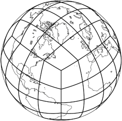
The atmospheric model’s horizontal grid is the so-called Cubed-Sphere grid (see Figure 2) first used in Sadourny (1972). Each cube face is mapped to the surface of the sphere with the equal-angle gnomonic projection (Rancic et al., 1996). The vertical grid/coordinate is an eta-type coordinate, following Simmons and Burridge (1981). The horizontal resolution is about 55 km and the model has 46 vertical levels, up to about 0.3 hPa.

Figure 2: Tiling the surface of the sphere with quadrilaterals. An inscribed cube is projected to the surface of the sphere. The faces of the cubed sphere are further subdivided to form a quadrilateral grid of the desired resolution. Coordinate lines from the gnomonic equal-angle projection are shown, see e.g. Sadourny (1972).

The horizontal and vertical grids of NEMO

In this operational, global configuration, NEMO uses, in the horizontal, an ORCA-family, curvilinear, tripolar, orthogonal grid (based on Mercator projection), which has a pole in the Southern Hemisphere, collocated with the geographic South Pole, and two poles placed on land in the Northern Hemisphere (in Siberia and Canada), in order to overcome the Pole singularities.

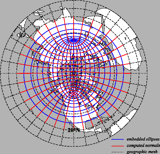
Figure 3: ORCA mesh conception. The departure from an isotropic Mercator grid start poleward of 20. The two "north pole" are the foci of a series of embedded ellipses (blue curves) which are determined analytically and form the i-lines of the ORCA mesh (pseudo latitudes). Then, following Madec and Imbard (1996), the normal to the series of ellipses (red curves) is computed which provide the j-lines of the mesh (pseudo longitudes).

The ORCA grid is based on the semi-analytical method of Madec and Imbard (1996). It allows to construct a global orthogonal curvilinear ocean mesh, which has no singularity point inside the computational domain, since two north mesh poles are introduced, in addition to the South Pole, and placed on land. The method involves defining an analytical set of mesh parallels in the stereographic polar plan, computing the associated set of mesh meridians and projecting the resulting mesh onto the sphere. The set of mesh parallels used is a series of embedded ellipses which foci are the two mesh north poles (see Figure 3). The resulting mesh presents no loss of continuity in either the mesh lines or the scale factors, or even the scale factor derivatives over the whole ocean domain, as the mesh is not a composite mesh. Poleward of 20°N, the two NH poles introduce a weak anisotropy over the ocean areas.

In the vertical, a partial step z-coordinate is used.

The horizontal resolution of the tri-polar grid is approximately 25 km and the ocean model has 50 vertical levels (31 in the first 500 m).

Post-processing output grid and re-gridding methods

The final output data are gridded on a regular lat-lon grid of 1x1°. Three-dimensional variables are provided on Standard Pressure Levels in the vertical. Surface fields are provided on the model’s orography, which is also an output field.

Re-gridding is performed through the ESMF package of NCL for CAM, CICE and NEMO. For CLM a re-gridding package included in CESM is used (for more information, see Sect. 2.6).

Initial Conditions and Initial Condition Perturbations

Initial condition (IC) fields for all necessary forecast modules (atmosphere, ocean, land and ice) are prepared routinely to initialize the monthly operational forecast. Additionally, a variety of perturbation techniques are applied to such initial conditions in order to obtain additional IC fields necessary to produce Ensemble Forecasts.

Atmospheric Initial Conditions and Perturbations

Atmospheric Initial Conditions (ICs) for operational forecasts are provided by ECMWF operational IFS 00UTC analyses for the first of the month as extracted from the MARS database on a regular lat-lon grid at ½° resolution. They are then interpolated onto the model quasi-regular cubed-sphere grid.

Nine further perturbed atmospheric initial conditions are obtained by applying a time-lagging technique, that is using previous ECMWF analyses at 12 hour intervals up to 5 days before. Before forecast integration, all time-lagged initial conditions are integrated for 12, 24, 36…hours, and so on up to 00UTC of the first of the month. This procedure finally provides 10 alternative atmospheric initial conditions from 00UTC of the first day of the month, all of them with superimposed perturbations of all model prognostic field variables provided by short-to-medium-range (12h up to 5 days) forecast errors.

In the case of hindcasts, ECMWF operational analyses are substituted by ERA5 analyses (Hersbach et al., 2020).

	Hindcasts	Forecasts
Atmosphere initialization	ERA5	ECMWF IFS operational
Atmosphere IC perturbations	10	10

Land Initial Condition and Perturbations

Land initial conditions are obtained from a one-month run ending on forecast initial date, forced by an observed atmosphere. This forced run is, in turn, initialized from a fixed 20-year spin-up run. Soil moisture and snow fields are also initialized from the same one-month forced run.

In order to generate three alternative land initial conditions, perturbations are obtained by using in turn re-analyses from ECMWF, NCEP and the mean of the two as forcing observed atmosphere. This provides three land initial conditions. In the case of operational forecasts, the observed atmosphere is provided by ECMWF operational analyses or by NCEP re-analyses or by a mean of both. In the case of hindcasts, the observed atmosphere is provided by ECMWF ERA-Interim or by NCEP re-analyses (Kalnay et al., 1996), or by a mean of both. This yields three possible initial conditions for the land surface.

For more ECMWF or NCEP Data Assimilation method details, see Sect. 2.6.

	Hindcasts	Forecasts
Land Initialization	Forced (obs. atmosphere) monthly run initialized from 10-years spin-up	Forced (obs. atmosphere) monthly run initialized from 10-years spin-up
Land IC perturbations	3	3
Soil moisture initialization	From land initialization	From land initialization
Snow initialization	From land initialization	From land initialization

Ocean Initial Condition and Perturbations

Ocean Initial Conditions are obtained by a 3D-VAR intermittent ocean data assimilation cycle performed with C-GLORS. Perturbations of initial conditions are obtained by re-assimilating 8 times (4 times in the case of hindcasts) observed data after insertion of added random perturbations on Sea-Level Anomalies (SLA) and on In-Situ profile observations of temperature and salinity (Burgers et al., 1998). At the same time, atmospheric fluxes and the ocean model equation of state (EOS) for seawater are also perturbed during the integration of the assimilating model (Brankart, 2013). Only in the case of real-time operational forecasts (not for hindcasts), the unperturbed control forecast is added to the 8 perturbed Ocean Initial Conditions (OICs), providing a total of 9 possible OICs to be combined with atmospheric and land ICs to generate the forecast ensemble.

	Hindcasts	Forecasts
Ocean initialization	C-GLORS	C-GLORS
Ocean IC perturbations	4	9

Sea-Ice Initial Condition and Perturbations

In order to produce Sea-Ice Initial Conditions, observed data of sea-ice concentration (SIC) and sea-ice-thickness (SIT) are assimilated, using on-line nudging schemes with a relaxation time scale of 8 hours and 5 days respectively. The observed SIC field is downloaded from the National Snow and Ice Data Center (NSIDC) (Cavalieri et al., 1999), while the SIT is constrained towards PIOMAS data (Pan-Arctic Ice Ocean Modeling and Assimilation System, Zhang and Rothrock, 2003) available for the Arctic area.

The assimilation of SIC and SIT data is performed during the C-GLORS ocean data-assimilation system, where, however, the LIM2 ice model within the NEMO ocean model substitutes the CICE4 used during coupled forecast integration. The LIM2 sea ice is the Louvain-la-Neuve Sea Ice Model (Fichefet and Morales Maqueda, 1997) which includes the representation of both thermodynamic and dynamic processes. The ice dynamics are calculated according to external forcing generated from wind stress, ocean stress and sea-surface tilt and to internal ice stresses. Internal ice stresses are computed using the elastic viscous-plastic (EVP) formulation of ice dynamics by Hunke and Dukowicz (1997) on a C-grid (Bouillon, Maqueda, Legat, and Fichefet, 2009).

No ice data are explicitly perturbed during data assimilation, however slightly different sea-ice data can be produced by the ocean data multiple perturbation procedure which generates the 9 alternative ocean initial conditions (4 for hindcasts). No Model dynamics or physics perturbations are applied to the sea-ice model and there is no special control forecast.

Combination and Choice of Perturbed Initial Conditions to generate the Ensemble

The 10 atmospheric perturbed ICs, the 3 land perturbed ICs and the 9 (4 in hindcast mode) ocean perturbed ICs are combined to yield 270 (120 in hindcast mode) possible perturbed ICs among which the 50 ICs (40 ICs in hindcast mode) to produce the forecast ensemble are chosen at random.

Forecast and Hindcast Ensemble Size and available initial dates

OP and POP Forecast ensemble size 50 members Hindcast ensemble size 40 members Hindcast coverage 1/1993-12/2016 with both SPS3 and SPS3.5 Pre-Operational (POP) Forecast coverage 1/2017-3/2018 with SPS3 Operational Forecasts (OP) coverage 4/2018-9/2020 with SPS3, 10/2020-present with SPS3.5

CMCC-SPS3.5 Summary Table of System Characteristics

</tr>

First date of implementation of the CMCC seasonal forecast system	January 1st, 2015
Date of implementation of the current version 3.5 of the CMCC seasonal forecast system	October 1st, 2020
Whether the system is a coupled ocean-atmosphere forecast system (Y/N)	Yes (CAM5.3, NEMO3.4, CLM4.5, CICE4)
Atmospheric model and its resolution	CAM5.3, 1/2° x 1/2° approximately
Oceanic model and its resolution	NEMO3.4, 1/4° x 1/4° approximately
Source of atmospheric initial conditions	ECMWF ERA5 (for hindcasts) ECMWF IFS (for forecasts)
Source of oceanic initial conditions	C-GLORS Global Ocean Intermittent 3D-VAR
Hindcast period	1/1993-12/2016
Ensemble size for hindcasts	40 members
Ensemble size for operational forecasts	50 members
Method of configuring the forecast ensemble	Progressive 12h backward time-lagged atmospheric analyses (10 perturbations, 5 days backward), 3 perturbed land analyses (different observed atmospheric forcing), 9 obs-data-perturbed ocean OI analyses for op-forecasts (4 for hindcasts), then random sample of 50 ensemble members among 270 possible combinations (120 for hindcasts)
Length of forecast	6 months
Data format	Netcdf and GRIB1
The latest date that predicted anomalies for the next month/season become available	8^th of each month
Method of construction of the forecast anomalies	Departures from model climate estimated from hindcasts dataset
URL where forecasts are displayed	https://sps.cmcc.it (public, with registration)
Point of contact	sps@cmcc.it

Table 1: CMCC-SPS3.5 Seasonal Forecasting System Characteristics

Provision of Global Forecasts Fields

The System is operated monthly (start date is first of the month) in Ensemble seasonal mode (6-month predictions, 50 ensemble members) and is completed by a database of monthly ensemble hindcasts (40 ensemble members) covering the period 1993-2016. This hindcasts database can be used to evaluate the performance of the system and to apply bias removal techniques from operational forecasts. The first operational seasonal forecast run produced for Copernicus-C3S, and contained in Copernicus-CDS, was initiated from April 1st, 2018, 00:00 UTC and monthly, from the first day of every month, since then. All further monthly seasonal forecasts (all with a forecast horizon of six months) from January 1st, 2017 until March 1st, 2018 are also available on Copernicus C3S-CDS as POPs, Pre-Operational Predictions. This constitutes, to date, a continuous database of 26 complete years of monthly ensemble seasonal (6-month) forecasts from January 1st, 1993 to the present date (December 2018). Further to this, CMCC has in fact been operating routine ensemble seasonal forecasts also with previous versions of the CMCC-SPS system since the year 2014.

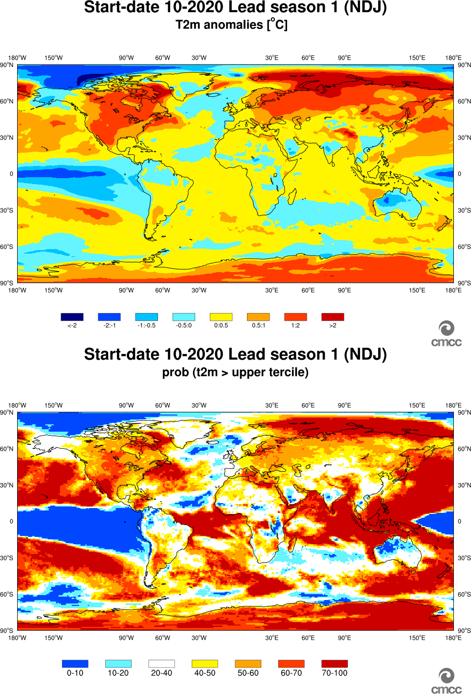
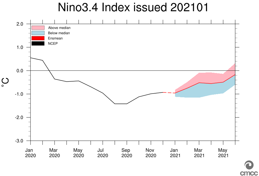
Figures 4 and 5 show an example of the global 2m Temperature and relative probability forecast (upper tercile) and of the El-Nino 3.4 index predicted by the operational seasonal forecast issued on October 1st, 2020 (lead season 1, 3-month mean).

Figure 4. CMCC-SPS3.5 Ensemble seasonal forecast from start date October 1st, 2020. 2m Temperature, three-month mean, lead season 1 (NDJ). Top: Ensemble mean. Bottom: Probability forecast to overcome the upper tercile. Anomalies are computed from the model’s own climate as computed from the 24-year database of hindcasts (1993-2016).

Figure 5. Nino 3.4 index forecast from start date October 1st, 2020 based on ensemble monthly means.

Provision of Verification Statistics

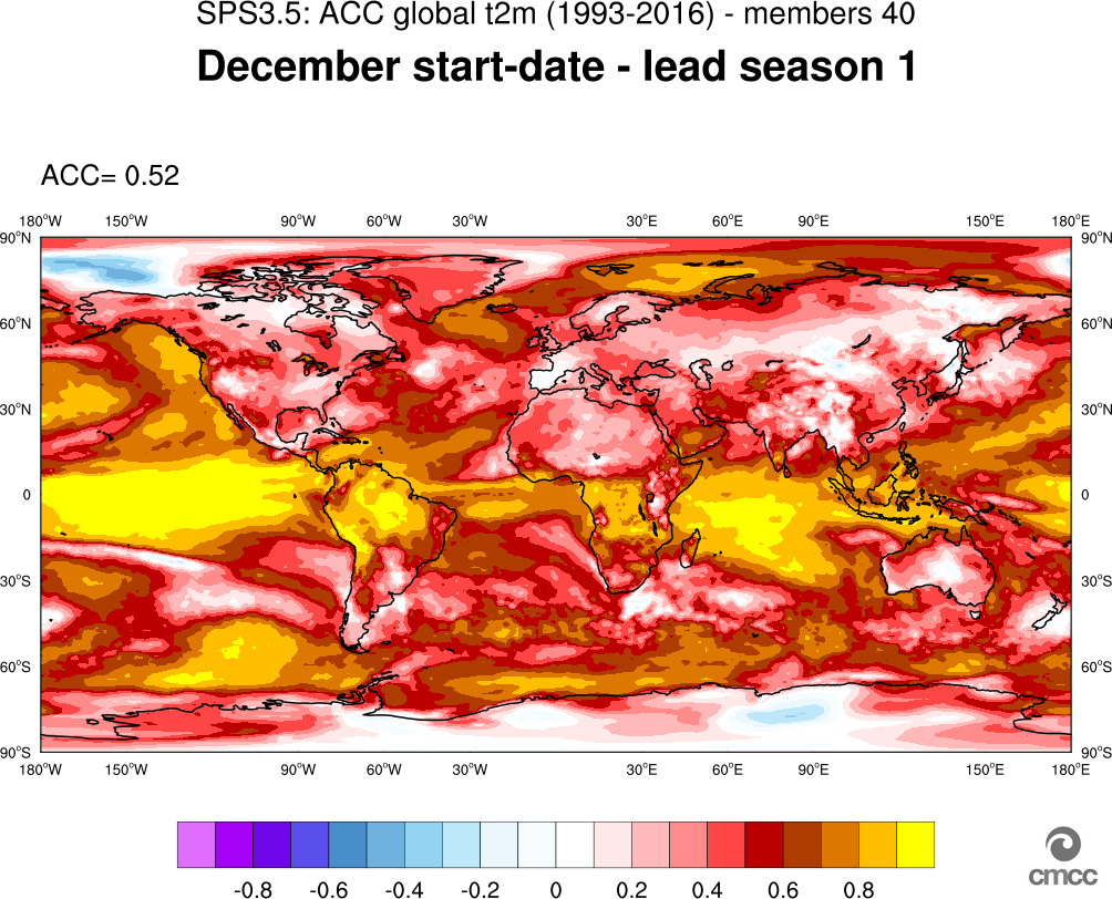
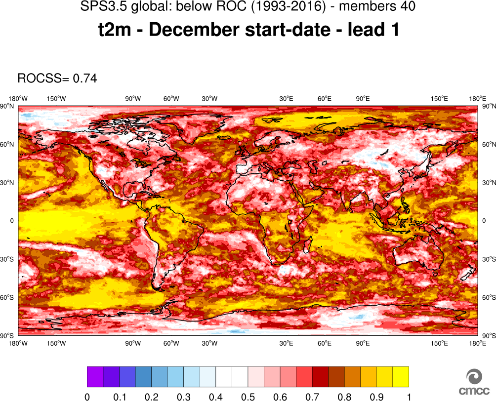
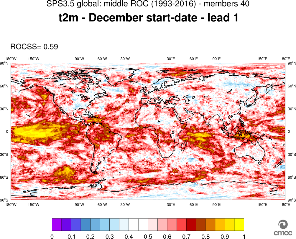
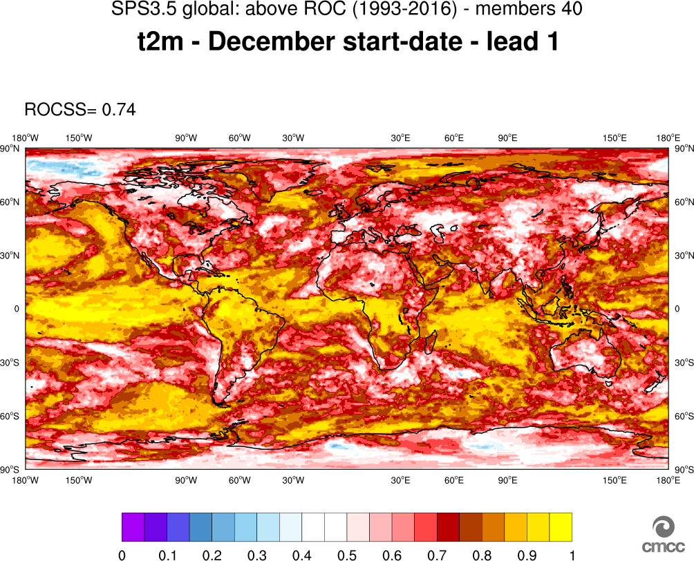
Before entering into operations and constantly thereafter, CMCC-SPS3 and SPS3.5 have been and are constantly the subject of extensive verification procedures and skill-scores computation. Such verification procedures include the computation and plot of a number of different metrics (e.g. Bias, RMS error, Anomaly Correlation Coefficient, ROC Score of, e.g., T2m and Precipitation on a global scale both for deterministic and probabilistic forecast. Figure 6 and Figure 7 show two examples of global fields of such metrics: Figure 6 shows the T2m Anomaly Correlation Coefficient (ACC) computed from all December 1st hindcasts, three-month mean for lead season 1 (JFM). Figure 7 shows the ROC Score for T2m, three month mean for lead season 1 (JFM), relative to lower, middle and upper terciles (Panels 7a, 7b and 7c, respectively).

Figure 6. Anomaly Correlation Coefficient (ACC) for 2m Temperature computed from all 24 years (1993-2016) December 1st hindcasts (40 members Ensembles), lead season 1.

Figure 7a. Relative Operating Characteristics (ROC) Score for 2m Temperature, lead season 1 relative to the lower tercile. ROC computed from all 24 years (1993-2016) December 1st hindcasts (40 members Ensembles).

Figure 7b. Relative Operating Characteristics (ROC) Score for 2m Temperature, lead season 1 relative to the middle tercile. ROC computed from all 24 years (1993-2016) December 1st hindcasts (40 members Ensembles).

Figure 7c. Relative Operating Characteristics (ROC) Score for 2m Temperature, lead season 1 relative to the upper tercile. ROC computed from all 24 years (1993-2016) December 1st hindcasts (40 members Ensembles).

Dissemination

Currently, CMCC Operational Real-Time Seasonal Forecasts and Verification Statistics are available on the public Copernicus Web-site for Seasonal Forecast products:

https://climate.copernicus.eu/seasonal-forecasts.

An alternative set of three-monthly mean products is currently also available on a public CMCC website at address https://sps.cmcc.it. A number of ensemble mean maps, ensemble spread, probability forecasts, Nino indices and past forecast scores are also available in graphical form on the same public access website.

In addition, CMCC Operational Real-Time Seasonal Forecasts and Verification Statistics are available on the WMO LC-LRFMME (WMO Lead Centre for Long-Range Forecast Multi-Model Ensemble) website at:

https://www.wmolc.org/index.php?sm_id=&tm_id=1&cdepth=2&upnum=1&ca_id=88&t1=1&s1=1

CMCC Seasonal Forecasts are also disseminated via the Mediterranean Outlook Forum (MEDCOF) Consensus Forecast and the Asian-Pacific Climate Center (APCC) Multi-Model System.

CMCC-SPS3.5 participation in Multi-Model Ensembles

CMCC Operational Seasonal Forecast is part of the following Multi Model Ensembles:

Copernicus Operational Multi-Model Forecasting System (C3S-CDS)
WMO LC-LRFMME (WMO Lead Centre for Long-Range Forecast Multi-Model Ensemble)
MEDCOF Multi-Model Consensus Forecast
APCC Multi-Model Ensemble Forecasting System

Where to find additional information

More extensive information on the Operational Forecast System Models can be found in the websites listed below.

More detailed documentation on CAM Model at: http://www.cesm.ucar.edu/models/cesm1.2/cam/

More detailed documentation on CLM Model at: http://www.cesm.ucar.edu/models/cesm1.2/clm/

More detailed documentation on NEMO Model at: https://www.nemo-ocean.eu/doc/

More ocean Data Assimilation details available at: http://c-glors.cmcc.it/index/index.html

More Data Assimilation details on ECMWF operational analysis documentation at: https://www.ecmwf.int/en/elibrary/16666-part-ii-data-assimilation

More Data Assimilation details on NCEP operational analysis and reanalyses documentation at: https://www.esrl.noaa.gov/psd/data/gridded/data.ncep.reanalysis2.html

Documentation on the system’s/models’ climatology and performance can be found at: https://www.cmcc.it/it/publications/rp0285-cmcc-sps3-the-cmcc-seasonal-prediction-system-3 and https://www.cmcc.it/wp-content/uploads/2020/09/TN0288-csp-09-2020-1.pdf

Documentation on the system’s new version (SPS3.5) retuning and effects on the model’s bias can be found at: https://www.cmcc.it/publications/tn290-tuning-of-some-orography-related-drag-parameterizations-in-the-atmospheric-component-of-the-cmcc-operational-seasonal-prediction-systems

More detailed documentation on the ESMF package of NCL at: https://www.ncl.ucar.edu/Applications/ESMF.shtml

More detailed documentation on the re-gridding package included in CESM at: http://www.cesm.ucar.edu/models/cesm1.2/clm/models/lnd/clm/doc/UsersGuide/book1.html

References

Bitz, C. M., and Lipscomb, W. H. (1999). A new energy-conserving sea ice model for climate study. J. Geophys. Res, 104(15), 669-15.

Brankart, J.-M. (2013). Impact of uncertainties in the horizontal density gradient upon low resolution global ocean modelling. Ocean Modell. 66, 64–76.
DOI: https://doi.org/10.1016/j.ocemod.2013.02.004

Branstetter, M.L., and James S. Famiglietti (1999). Testing the sensitivity of GCM-simulated runoff to climate model resolution using a parallel river transport algorithm. Proceedings of 14th Conference on Hydrology, American Meteorological Society, Dallas, Texas.

Branstetter, M.L. (2001). Development of a parallel river transport algorithm and applications to climate studies. University of Texas.

Bretherton, C. S., and S. Park (2009). A new moist turbulence parameterization in the community atmosphere mode, J. Climate, 22, 3422–3448, 2009a.

Bretherton, C.S., M. G. Flanner, and D. Mitchell (2012). Toward a minimal representation of aerosols in climate models: description and evaluation in the Community Atmosphere Model CAM5. Geosci. Model Dev., 5(3):709–739, 2012. doi: 10.5194/gmd-5-709-2012

Briegleb, B. P., & Light, B. (2007). A Delta-Eddington multiple scattering parameterization for solar radiation in the sea ice component of the Community Climate System Model. NCAR Tech. Note NCAR/TN-472+ STR, 100.

Bouillon, S., M.M. Maqueda, V. Legat, and T. Fichefet. (2009) An elastic-viscousplastic sea ice model formulated on Arakawa b and c grids. Ocean Modelling, 27:174–184.

Burgers, G., van Leeuwen, P.J., Evensen, G. 1998. Analysis scheme in the ensemble Kalman filter. Mon. Weather Rev. 126, 1719–1724.
http://dx.doi.org/10.1175/1520-0493(1998)126<1719:ASITEK>2.0.CO;2.

Cavalieri, D. J., Parkinson, C. L., Gloersen, P., Comiso, J. C., and Zwally, H. J. (1999). Deriving long-term time series of sea ice cover from satellite passive-microwave multisensor data sets, J. Geophys. Res., 104, 15803–15814, doi:10.1029/1999JC900081

Craig, A. P., Vertenstein, M., & Jacob, R. (2011). A new flexible coupler for earth system modeling developed for CCSM4 and CESM1. International Journal of High Performance Computing Applications, 1094342011428141.

Davoli, G., S. Tibaldi, A. Sanna, M. Benassi, A. Borrelli, A. Cantelli, M. del Mar Chaves Montero and S. Gualdi (2021). Tuning of some orography-related drag parameterizations in the atmospheric component of the CMCC Operational Seasonal Prediction System. CMCC Technical Note TN0290. Available from https://www.cmcc.it/publications/tn290-tuning-of-some-orography-related-drag-parameterizations-in-the-atmospheric-component-of-the-cmcc-operational-seasonal-prediction-systems. Also, submitted to Bull. Atmos. Sci. and Tech.

Dee, D., et al. (2011). The ERA-Interim reanalysis: configuration and performance of the data assimilation system. Q. J. R. Meteorol. Soc., 137, 553–597.

Dennis, J.M. et al. (2012). “CAM-SE: A scalable spectral element dynamical core for the Community Atmosphere Model”. In: The International Journal of High Performance Computing Applications 26.

Fichefet T. and M.A. Morales Maqueda (1997). Sensitivity of a global sea ice model to the treatment of ice thermodynamics and dynamics. Journal of Geophysical Research, 102:12609–12646, 1997.

Flanner, M.G., et al. (2007). Present-day climate forcing and response from black carbon snow. Journal of Geophysical Research: Atmospheres. 112, D11.

Gaspar, P., Y. Gregoris, and J.-M. Lefevre (1990). A simple eddy kinetic energy model for simulations of the oceanic vertical mixing Tests at station papa and long-term upper ocean study site. J. Geophys. Res, 95 (C9).

Gettelman, A., H. Morrison, and S.J. Ghan (2008). A new two-moment bulk stratiform cloud microphysics scheme in the Community Atmosphere Model, version 3 (CAM3). Part II: Single-column and global results.” Journal of Climate 21(15): 3660-3679.

Griffies, S. (2004). Fundamentals of ocean climate models. Princeton University Press, 434pp.

Gualdi, S., A. Borrelli, S. Davoli, M. del Mar Chaves Montero, S. Masina, A. Navarra, A. Sanna, S. Tibaldi (2020). The new CMCC Operational Seasonal Prediction System SPS3.5, CMCC Technical Note RP0288, https://doi.org/10.25424/CMCC/SPS3.5.

Holland, M.M., D. A. Bailey, B. P. Briegleb, B. Light, and E. Hunke (2012). Improved sea ice shortwave radiation physics in CCSM4: the impact of melt ponds and aerosols on Arctic sea ice. J. Climate, 25(5): 1413–1430, 2012. doi:10.1175/ JCLI-D-11-00078.1.

Hunke, E. C., and Dukowicz, J. K. (1997). An elastic-viscous-plastic model for sea ice dynamics. Journal of Physical Oceanography, 27(9), 1849-1867.

Hunke, E. C., Lipscomb, W. H., & Turner, A. K. (2010). CICE: the Los Alamos Sea Ice Model Documentation and Software User’s Manual Version 4.1 LA-CC-06-012. T-3 Fluid Dynamics Group, Los Alamos National Laboratory, 675.

Hurrell, James W., et al. (2013). The community earth system model: a framework for collaborative research. Bulletin of the American Meteorological Society 94(9):1339-1360.

Iacono M.J., J. S. Delamere, E. J. Mlawer, M. W. Shephard, S. A. Clough, and W. D. Collins (2008). Radiative forcing by long-lived greenhouse gases: Calculations with the AER radiative transfer models, J. Geophys. Res.: Atmospheres, 113(D13). doi:10.1029/2008JD009944.

IPCC (2013). Climate Change: The Physical Science Basis. Contribution of Working Group I to the Fifth Assessment Report of the Intergovernmental Panel on Climate Change [Stocker, T.F., D. Qin, G.-K. Plattner, M. Tignor, S.K. Allen, J. Boschung, A. Nauels, Y. Xia, V. Bex and P.M. Midgley (eds.)]. Cambridge University Press, Cambridge, United Kingdom and New York, NY, USA, 1535 pp, doi:10.1017/CBO9781107415324.

Kalnay, E., Kanamitsu, M., Kistler, R., Collins, W., Deaven, D., Gandin, L., … & Zhu, Y. (1996). The NCEP/NCAR 40-year reanalysis project. Bulletin of the American Meteorological Society, 77(3), 437-471.

Liu X., R. C. Easter, S. J. Ghan, R. Zaveri, P. Rasch, X. Shi, J.-F. Lamarque, A. Get- telman, H. Morrison, F. Vitt, A. Conley, S. Park, R. Neale, C. Hannay, A. M. L. Ekman, P. Hess, N. Mahowald, W. Collins, M. J. Iacono, C. S. (2012). Toward a minimal rep- resentation of aerosols in climate models: description and evaluation in the Community Atmosphere Model CAM5. Geosci. Model Dev., 5(3):709–739. doi: 10.5194/gmd-5-709-2012.

Madec, G., and M. Imbard (1996). A global ocean mesh to overcome the north pole singularity. Clim. Dyn., 12, 381-388.

Madec, G. et al (2008). NEMO ocean engine. Institut Pierre Simon Laplace, Note du Pole de Modelisation 27, 2008. URL: http://www.nemo-ocean.eu/content/download/21612/97924/file/NEMO_book_3_4.pdf

Neale R.B. and Coauthors (2012). Description of the NCAR Community Atmosphere Model (CAM 5.0). NCAR Technical Note NCAR/TN-486, National Center for Atmospheric Research. URL: http://www.cesm.ucar.edu/models/cesm1.1/cam/docs/description/cam5_desc.pdf.

Oleson, K. W., et al. (2013). Technical description of version 4.5 of the Community Land Model (CLM). NCAR Tech. Note NCAR/TN-503+ STR. National Center for Atmospheric Research, Boulder, CO, 422 pp. doi: 10.5065/D6RR1W7M

Park. S. and C. S. Bretherton (2009). The University of Washington shallow convection and moist turbulence schemes and their impact on climate simulations with the Community Atmosphere Model. J. Climate, 22(12):3449–3469, 2009. doi:10. 1175/2008JCLI2557.1.

Patera A.T. (1984). A spectral element method for fluid dynamics - Laminar flow in a channel expansion. Journal of Computational Physics, 54:468–488, 1984.

Pincus, R., H. W. Barker, and J.-J. Morcrette (2003). A fast, flexible, approximate technique for computing radiative transfer in inhomogeneous cloud fields. J. Geophys. Res.: Atmospheres, 108(D13), 2003. doi: 10.1029/2002JD003322.

Rancic, M., R. Purser, and F. Mesinger (1996). A global shallow-water model using an expanded spherical cube: Gnomonic versus conformal coordinates, Q. J. R. Meteorol. Soc., 122, 959–982.

Raymond, D. J., and A. M. Blyth (1986). A stochastic mixing model for non-precipitating cumulus clouds, J. Atmos. Sci., 43, 2708–2718.

Raymond, D. J., and A. M. Blyth (1992). Extension of the stochastic mixing model to cumulonimbus clouds, J. Atmos. Sci., 49, 1968–1983.

Richter, J. H., A. Solomon and J.T. Bacmeister (2014). Effects of vertical resolution and nonorographic gravity wave drag on the simulated climate in the Community Atmosphere Model, version 5. Journal of Advances in Modeling Earth Systems, 6(2), 357-383.

Richter, J. H., and P. J. Rasch (2008). Effects of convective momentum transport on the atmospheric circulation in the community atmosphere model, version 3, J. Climate, 21, 1487–1499, 2008.

Sanna, A., A. Borrelli, P. Athanasiadis, S. Materia, A. Storto, S. Tibaldi, S. Gualdi (2017). CMCC-SPS3: CMCC-SPS3: The CMCC Seasonal Prediction System 3. Centro Euro-Mediterraneo sui Cambiamenti Climatici. CMCC Tech. Rep. RP0285, 61pp. Available at adress: https://www.cmcc.it/it/publications/rp0285-cmcc-sps3-the-cmcc-seasonal-prediction-system-3/

Sadourny, R. (1972): Conservative finite-difference approximations of the primitive equations on quasi uniform spherical grids, Mon. Wea. Rev., 100 (2), 136–144.

Simmons, A. J., and D. M. Burridge (1981): An energy and angular momentum conserving vertical finite-difference scheme and hybrid vertical coordinates, Mon. Wea. Rev., 109, 758–766.

Simmons, H. L., S. R. Jayne, L. C. St. Laurent, and A. J. Weaver (2004). Tidally driven mixing in a numerical model of the ocean general circulation. Ocean Modelling, 245–263.

Subin, Z. M., Riley, W. J., & Mironov, D. (2012). An improved lake model for climate simulations: Model structure, evaluation, and sensitivity analyses in CESM1. Journal of Advances in Modeling Earth Systems, 4(1).

Swenson, S. C., Lawrence, D. M., & Lee, H. (2012). Improved simulation of the terrestrial hydrological cycle in permafrost regions by the Community Land Model. Journal of Advances in Modeling Earth Systems, 4(3).

Zalesak, S. T. (1979). Fully multidimensional flux corrected transport algorithms for fluids. J. Comput. Phys., 31.

Zhang, J. L. and Rothrock, D. A. (2003). Modeling global sea ice with a thickness and enthalpy distribution model in generalized curvilinear coordinates, Mon. Weather Rev., 131, 845–861.

Zhang, G. J., and N. A. McFarlane (1995). Sensitivity of climate simulations to the parameterization of cumulus convection in the Canadian Climate Centre general circulation model, Atmosphere-Ocean, 33, 407–446.